在浏览器中使用TensorFlow.js的好处
- 交互性-浏览器有许多工具可以可视化正在进行的过程(图形,动画等);
- 传感器-浏览器可以直接访问设备的传感器(相机,GPS,加速度计等);
- 用户数据的安全性-无需将处理后的数据发送到服务器;
- 与用Python创建的模型兼容。
性能
主要问题之一是性能。
由于事实上机器学习正在使用类似矩阵的数据(张量)执行各种数学运算,因此浏览器中用于此类计算的库使用WebGL。如果在纯JS中执行相同的操作,则可以显着提高性能。自然,如果由于某种原因浏览器不支持WebGL,该库会有一个后备功能(在撰写本文时,caniuse显示97.94%的用户支持WebGL)。
为了提高性能,Node.js将本机绑定与TensorFlow结合使用。在这里,CPU,GPU和TPU(张量处理单元)可以用作加速器
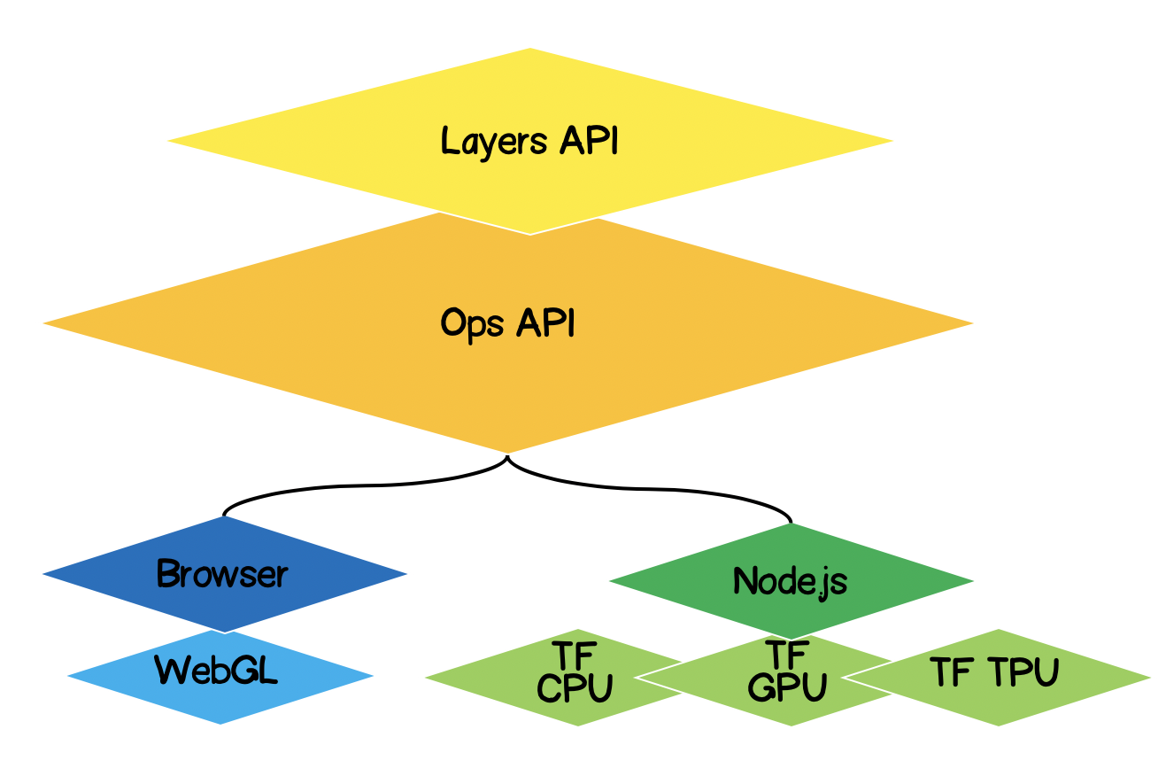
TensorFlow.js架构
- 最低层-在张量上执行数学运算时,此层负责并行计算。
- Ops API-提供用于在张量上执行数学运算的API。
- Layers API-允许您使用不同类型的层(密集层,卷积层)创建复杂的神经网络模型。该层类似于Keras Python API,并且能够加载基于Keras Python的预训练网络。
问题的提法
对于给定的实验点集,必须找到近似线性函数的方程。换句话说,我们需要找到一条最接近实验点的线性曲线。

解决方案形式化
任何机器学习的核心都是模型,在我们的例子中,这是线性函数的方程式:
根据条件,我们还有一组实验点:
假设 第j个训练步骤中,计算了线性方程的以下系数。现在我们需要用数学方法表达所选系数的准确性。为此,我们需要计算误差(损失),例如可以通过标准偏差确定误差。Tensorflow.js提供了一组常用的损失函数:tf.metrics.meanAbsoluteError,tf.metrics.meanSquaredError等。
近似的目的是使误差函数最小化 。让我们为此使用梯度下降方法。有必要:
- -通过计算相对于系数的偏导数来找到矢量梯度 ;
- -在与梯度矢量相反的方向上校正方程式的系数。因此,我们将最小化误差函数:
是学习率,是模型的可调参数之一。对于梯度下降,它在整个学习过程中不会改变。较小的学习率值可能导致模型的学习过程长时间收敛,并且可能会导致局部最小值发生碰撞(图2),而较大的值可能会导致训练的每个步骤的误差值无限增大(图1)。
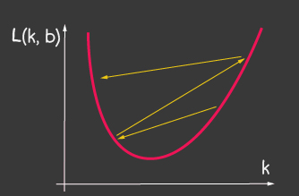
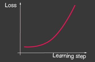
|


|
|---|---|
| 图1:高学习率的价值 | 图2:小学习率 |
如何在没有Tensorflow.js的情况下实现它
例如,计算损失函数的值(标准偏差)如下所示:
function loss(ysPredicted, ysReal) {
    const squaredSum = ysPredicted.reduce(
        (sum, yPredicted, i) => sum + (yPredicted - ysReal[i]) ** 2,
        0);
    return squaredSum / ysPredicted.length;
}
但是,输入数据量可能很大。在模型训练期间,我们不仅需要计算每次迭代中损失函数的值,还需要执行更严格的操作-计算梯度。因此,使用tensorflow是有意义的,它可以使用WebGL优化计算。而且,代码变得更具表现力,比较一下:
    function loss(ysPredicted, ysReal) => {
        const ysPredictedTensor = tf.tensor(ysPredicted);
        const ysRealTensor = tf.tensor(ysReal);
        const loss = ysPredictedTensor.sub(ysRealTensor).square().mean();
        return loss.dataSync()[0];
    };
TensorFlow.js解决方案
好消息是,我们将不必为给定的误差函数(损失)编写优化器,也不会开发用于计算偏导数的数值方法,我们已经为我们实现了反向传播算法。我们只需要遵循以下步骤:
- 设置模型(在我们的示例中为线性函数);
- 描述误差函数(在我们的例子中,这是标准偏差)
- 选择一种已实现的优化器(可以使用您自己的实现来扩展库)
什么是张量
绝对每个人都在数学上遇到过张量-它们是标量,向量,2D-矩阵,3D-矩阵。张量是以上所有内容的广义概念。它是一个数据容器,其中包含同构类型的数据(tensorflow支持int32,float32,bool,complex64,string),并具有特定的形状(轴数(行数)和每个轴中的元素数)。下面我们将考虑到3D矩阵的张量,但是由于这是一个概括,张量可以具有任意数量的轴:5D,6D,... ND。
TensorFlow具有以下用于张量生成的API:
tf.tensor (values, shape?, dtype?)其中shape是张量的形状并由一个数组给出,其中元素的数量是轴的数量,数组的每个值确定沿每个轴的元素的数量。例如,要定义一个4x2矩阵(4行2列),该表单将采用[4,2]的形式。
| 可视化 | 描述 |
|---|---|

|
标量
等级:0 形式:[] JS结构: TensorFlow API: |

|
矢量
等级:1 形状:[4] JS结构: TensorFlow API: |
 |
矩阵
等级:2 形状:[4,2] JS结构: TensorFlow API: |
 |
矩阵
等级:3 形状:[4,2,3] JS结构: TensorFlow API: |
使用TensorFlow.js进行线性逼近
最初,我们将讨论使代码可扩展。我们可以通过任何一种函数将线性近似转换为实验点的近似。类的层次结构如下所示:

让我们开始实现抽象类的方法,除了将在子类中定义的抽象方法之外,如果由于某种原因该方法未在子类中定义,则这里我们将仅保留带有错误的存根。
import * as tf from '@tensorflow/tfjs';

export default class AbstractRegressionModel {
    constructor(
        width,
        height,
        optimizerFunction = tf.train.sgd,
        maxEpochPerTrainSession = 100,
        learningRate = 0.1,
        expectedLoss = 0.001
    ) {
        this.width = width;
        this.height = height;
        this.optimizerFunction = optimizerFunction;
        this.expectedLoss = expectedLoss;
        this.learningRate = learningRate;
        this.maxEpochPerTrainSession = maxEpochPerTrainSession;

        this.initModelVariables();

        this.trainSession = 0;
        this.epochNumber = 0;
        this.history = [];
    }
}因此,在模型的构造函数中,我们定义了宽度和高度-这些是我们将在其上放置实验点的平面的实际宽度和高度。这对于标准化输入数据是必需的。那些。如果我们有,然后进行标准化后,我们将拥有:
optimizerFunction-我们将使优化器的任务更加灵活,以便能够尝试库中可用的其他优化器,默认情况下,我们将随机梯度下降方法设置为tf.train.sgd。我还建议您与其他可用的优化程序一起使用,这些优化程序可以在训练期间调整learningRate,并且学习过程得到了极大的改善,例如,尝试以下优化程序:tf.train.momentum,tf.train.adam。
这样的学习过程不是无止境的,我们已经定义了两个参数maxEpochPerTrainSesion和expectedLoss-通过这种方式,我们将在达到最大训练迭代次数或误差函数的值变得小于预期误差时停止训练过程(我们将在下面的训练方法中考虑所有因素)。
在构造函数中,我们调用initModelVariables方法-但按照约定,稍后在子类中对它进行存根和定义。
initModelVariables() {
    throw Error('Model variables should be defined')
}
现在让我们实现火车模型的主要方法:
/**
     * Train model until explicitly stop process via invocation of stop method
     * or loss achieve necessary accuracy, or train achieve max epoch value
     *
     * @param x - array of x coordinates
     * @param y - array of y coordinates
     * @param callback - optional, invoked after each training step
     */
    async train(x, y, callback) {
        const currentTrainSession = ++this.trainSession;
        this.lossVal = Number.POSITIVE_INFINITY;
        this.epochNumber = 0;
        this.history = [];

        // convert array into tensors
        const input = tf.tensor1d(this.xNormalization(x));
        const output = tf.tensor1d(this.yNormalization(y));

        while (
            currentTrainSession === this.trainSession
            && this.lossVal > this.expectedLoss
            && this.epochNumber <= this.maxEpochPerTrainSession
            ) {
            const optimizer = this.optimizerFunction(this.learningRate);
            optimizer.minimize(() => this.loss(this.f(input), output));
            this.history = [...this.history, {
                epoch: this.epochNumber,
                loss: this.lossVal
            }];
            callback && callback();
            this.epochNumber++;
            await tf.nextFrame();
        }
    }
如果外部API调用train方法,而先前的训练课程尚未结束,trainSession本质上是训练课程的唯一标识符。
从代码中可以看到,我们是从一维数组创建tensor1d的,虽然必须首先对数据进行规范化,但是规范化的功能如下:
xNormalization = xs => xs.map(x => x / this.width);
yNormalization = ys => ys.map(y => y / this.height);
yDenormalization = ys => ys.map(y => y * this.height);
在一个循环中,对于每个训练步骤,我们都需要将损失函数传递给模型优化器。按照约定,损失函数将由标准偏差设置。然后使用tensorflow.js API,我们可以:
    /**
     * Calculate loss function as mean-square deviation
     *
     * @param predictedValue - tensor1d - predicted values of calculated model
     * @param realValue - tensor1d - real value of experimental points
     */
    loss = (predictedValue, realValue) => {
        // L = sum ((x_pred_i - x_real_i)^2) / N
        const loss = predictedValue.sub(realValue).square().mean();
        this.lossVal = loss.dataSync()[0];
        return loss;
    };
学习过程继续
- 不会达到迭代次数的限制
- 无法达到所需的错误精度
- 新的培训过程尚未开始
还要注意损失函数的调用方式。为了获得预测值-我们将其称为函数f-实际上将根据执行回归的方式设置形式,并在抽象类中按约定放置一个存根:
  f(x) {
        throw Error('Model should be defined')
  }
在训练的每个步骤中,在历史模型对象的属性中,我们保存每个训练时期的误差变化动态。
在训练模型的过程之后,我们需要一种方法来接受输入并使用训练后的模型输出计算出的输出。为此,我们在API中定义了Forecast方法,它看起来像这样:
/**
     * Predict value basing on trained model
     *  @param x - array of x coordinates
     *  @return Array({x: integer, y: integer}) - predicted values associated with input
     *
     * */
    predict(x) {
        const input = tf.tensor1d(this.xNormalization(x));
        const output = this.yDenormalization(this.f(input).arraySync());
        return output.map((y, i) => ({ x: x[i], y }));
    }
请注意arraySync,类似于node.js,如果有arraySync方法,则肯定有一个异步数组方法返回Promise。这里需要承诺,因为正如我们之前所说,张量都被迁移到WebGL以加快计算速度,并且该过程变得异步,因为将数据从WebGL移至JS变量需要时间。
我们完成了一个抽象类,您可以在此处查看代码的完整版本:
AbstractRegressionModel.js
import * as tf from '@tensorflow/tfjs';

export default class AbstractRegressionModel {

    constructor(
        width,
        height,
        optimizerFunction = tf.train.sgd,
        maxEpochPerTrainSession = 100,
        learningRate = 0.1,
        expectedLoss = 0.001
    ) {
        this.width = width;
        this.height = height;
        this.optimizerFunction = optimizerFunction;
        this.expectedLoss = expectedLoss;
        this.learningRate = learningRate;
        this.maxEpochPerTrainSession = maxEpochPerTrainSession;

        this.initModelVariables();

        this.trainSession = 0;
        this.epochNumber = 0;
        this.history = [];
    }

    initModelVariables() {
        throw Error('Model variables should be defined')
    }

    f() {
        throw Error('Model should be defined')
    }

    xNormalization = xs => xs.map(x => x / this.width);
    yNormalization = ys => ys.map(y => y / this.height);
    yDenormalization = ys => ys.map(y => y * this.height);

    /**
     * Calculate loss function as mean-squared deviation
     *
     * @param predictedValue - tensor1d - predicted values of calculated model
     * @param realValue - tensor1d - real value of experimental points
     */
    loss = (predictedValue, realValue) => {
        const loss = predictedValue.sub(realValue).square().mean();
        this.lossVal = loss.dataSync()[0];
        return loss;
    };

    /**
     * Train model until explicitly stop process via invocation of stop method
     * or loss achieve necessary accuracy, or train achieve max epoch value
     *
     * @param x - array of x coordinates
     * @param y - array of y coordinates
     * @param callback - optional, invoked after each training step
     */
    async train(x, y, callback) {
        const currentTrainSession = ++this.trainSession;
        this.lossVal = Number.POSITIVE_INFINITY;
        this.epochNumber = 0;
        this.history = [];

        // convert data into tensors
        const input = tf.tensor1d(this.xNormalization(x));
        const output = tf.tensor1d(this.yNormalization(y));

        while (
            currentTrainSession === this.trainSession
            && this.lossVal > this.expectedLoss
            && this.epochNumber <= this.maxEpochPerTrainSession
            ) {
            const optimizer = this.optimizerFunction(this.learningRate);
            optimizer.minimize(() => this.loss(this.f(input), output));
            this.history = [...this.history, {
                epoch: this.epochNumber,
                loss: this.lossVal
            }];
            callback && callback();
            this.epochNumber++;
            await tf.nextFrame();
        }
    }

    stop() {
        this.trainSession++;
    }

    /**
     * Predict value basing on trained model
     *  @param x - array of x coordinates
     *  @return Array({x: integer, y: integer}) - predicted values associated with input
     *
     * */
    predict(x) {
        const input = tf.tensor1d(this.xNormalization(x));
        const output = this.yDenormalization(this.f(input).arraySync());
        return output.map((y, i) => ({ x: x[i], y }));
    }
}
对于线性回归,我们定义了一个将从抽象类继承的新类,在该类中,我们只需要定义两个方法initModelVariables和f即可。
由于我们正在进行线性逼近,因此必须指定两个变量k,b-它们将是标量张量。对于优化器,我们必须指出它们是可定制的(变量),并分配任意数字作为初始值。
initModelVariables() {
   this.k = tf.scalar(Math.random()).variable();
   this.b = tf.scalar(Math.random()).variable();
}在这里考虑变量的API :
tf.variable (initialValue, trainable?, name?, dtype?)请注意trainable的第二个参数-一个布尔变量,默认情况下为true。它由优化器使用,它告诉他们在最小化损失函数时是否有必要配置此变量。当我们基于从Keras Python下载的预训练模型构建新模型时,这很有用,并且我们确信无需重新训练此模型中的某些层。
接下来,我们需要使用tensorflow API定义近似函数的方程式,看一下代码,您将直观地了解如何使用它:
f(x) {
   // y = kx + b
   return  x.mul(this.k).add(this.b);
}
例如,通过这种方式,您可以指定二次近似:
initModelVariables() {
   this.a = tf.scalar(Math.random()).variable();
   this.b = tf.scalar(Math.random()).variable();
   this.c = tf.scalar(Math.random()).variable();
}

f(x) {
    // y = ax^2 + bx + c
    return this.a.mul(x.square()).add(this.b.mul(x)).add(this.c);
}
在这里,您可以查看线性和二次回归模型:
LinearRegressionModel.js
import * as tf from '@tensorflow/tfjs';
import AbstractRegressionModel from "./AbstractRegressionModel";

export default class LinearRegressionModel extends AbstractRegressionModel {
    initModelVariables() {
        this.k = tf.scalar(Math.random()).variable();
        this.b = tf.scalar(Math.random()).variable();
    }

    f = x => x.mul(this.k).add(this.b);
}
QuadraticRegressionModel.js
import * as tf from '@tensorflow/tfjs';
import AbstractRegressionModel from "./AbstractRegressionModel";

export default class QuadraticRegressionModel extends AbstractRegressionModel {
    initModelVariables() {
        this.a = tf.scalar(Math.random()).variable();
        this.b = tf.scalar(Math.random()).variable();
        this.c = tf.scalar(Math.random()).variable();
    }

    f = x => this.a.mul(x.square()).add(this.b.mul(x)).add(this.c);
}
下面是用React编写的一些代码,这些代码使用书面的线性回归模型并为用户创建UX:
Regression.js
import React, { useState, useEffect } from 'react';

import Canvas from './components/Canvas';
import LossPlot from './components/LossPlot_v3';
import LinearRegressionModel from './model/LinearRegressionModel';

import './RegressionModel.scss';

const WIDTH = 400;
const HEIGHT = 400;
const LINE_POINT_STEP = 5;

const predictedInput = Array.from({ length: WIDTH / LINE_POINT_STEP + 1 })
    .map((v, i) => i * LINE_POINT_STEP);

const model = new LinearRegressionModel(WIDTH, HEIGHT);

export default () => {
    const [points, changePoints] = useState([]);
    const [curvePoints, changeCurvePoints] = useState([]);
    const [lossHistory, changeLossHistory] = useState([]);

    useEffect(() => {
        if (points.length > 0) {
            const input = points.map(({ x }) => x);
            const output = points.map(({ y }) => y);

            model.train(input, output, () => {
                changeCurvePoints(() => model.predict(predictedInput));
                changeLossHistory(() => model.history);
            });
        }
    }, [points]);

    return (
        <div className="regression-low-level">
            <div className="regression-low-level__top">
                <div className="regression-low-level__workarea">
                    <div className="regression-low-level__canvas">
                        <Canvas
                            width={WIDTH}
                            height={HEIGHT}
                            points={points}
                            curvePoints={curvePoints}
                            changePoints={changePoints}
                        />
                    </div>
                    <div className="regression-low-level__toolbar">
                        <button
                            className="btn btn-red"
                            onClick={() => model.stop()}>Stop
                        </button>
                        <button
                            className="btn btn-yellow"
                            onClick={() => {
                                model.stop();
                                changePoints(() => []);
                                changeCurvePoints(() => []);
                            }}>Clear
                        </button>
                    </div>
                </div>
                <div className="regression-low-level__loss">
                    <LossPlot
                              loss={lossHistory}/>
                </div>

            </div>
        </div>
    )
}
结果:
我强烈建议您执行以下任务:
- 通过对数函数实现函数逼近
- 对于tf.train.sgd优化器,请尝试使用learningRate并观察学习过程如何变化。尝试将learningRate设置得很高,以得到如图2所示的图片。
- 将优化器设置为tf.train.adam。学习过程是否有所改善?学习过程是否取决于更改模型构造函数中的learningRate值。